Huffman Coding Builds Optimal Trees for Lossless Data

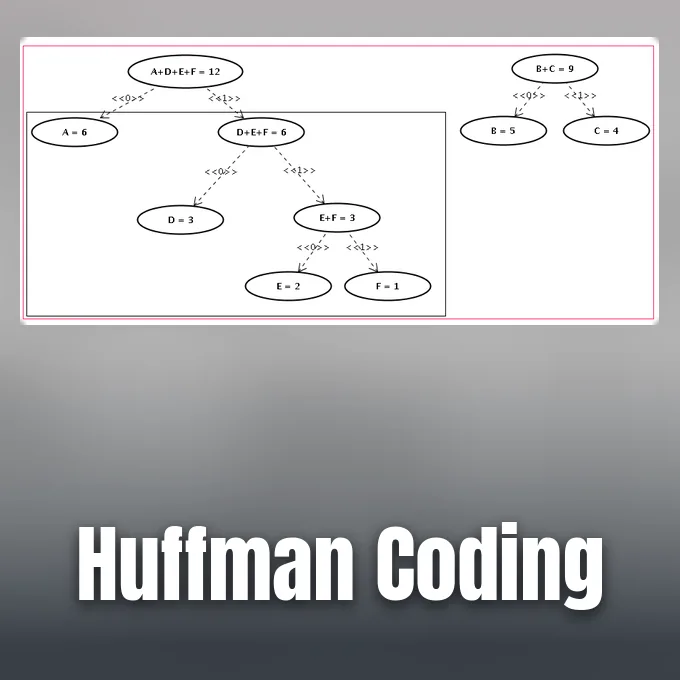
Learning how Huffman coding works reveals the mathematical foundations of lossless data compression in computer systems. Graduate student David A. Huffman developed the technique at the Massachusetts Institute of Technology in 1951 during an information theory course taught by Professor Robert M. Fano. Older formats assign identical bit counts to every character, but Huffman’s procedure calculates variable-length binary codes based on observed symbol frequencies. It builds an optimal prefix-free tree from the bottom up so that common characters receive shorter digital representations [16].

Origins of the Minimum Redundancy Problem

David A. Huffman faced an academic dilemma at the Massachusetts Institute of Technology in 1951. Professor Robert M. Fano offered his graduate class a choice between a final examination or a term paper on designing the most efficient binary code. Huffman worked for months without finding an optimal proof and prepared to throw his notes into the trash to study for the exam [10].

An epiphany struck Huffman just as he discarded his papers. He realized that building a tree from the bottom up, combining the least probable symbols toward the root, guarantees an optimal code. Professor Robert M. Fano and Claude Shannon had tried working top down from the root, yielding suboptimal results. When Huffman showed his proof, Fano exclaimed, “Is that all there is to it!”. A profile in the September 1991 issue of Scientific American on pages 54 and 58 noted that Huffman solved what senior scholars could not [10].

Huffman published his breakthrough in 1952 under the title A Method for the Construction of Minimum-Redundancy Codes [14]. Stanford University professor Donald E. Knuth praised it as a foundational concept in computing. In 1967, Huffman moved to the University of California at Santa Cruz to chair computer science, where at age 65 he continued teaching digital signal processing [10].

Variable Length Codes and How Huffman Coding Works

The operational logic of how Huffman coding works centers on building a variable-length prefix code that assigns short bit patterns to frequent characters and longer patterns to rare characters. Standard ASCII text stores every letter, numeral, and punctuation mark as a fixed sequence of eight bits, regardless of frequency. By allowing codeword lengths to vary according to empirical frequencies, a compression encoder reduces the total bits required to store or transmit text [11].

A classic demonstration from Rosetta Code analyzes the sample sentence “this is an example for huffman encoding”. In this sample phrase, the space character appears 6 times and receives the three-bit code 101. The letter n appears 4 times and receives code 010, while the characters a, e, and f each occur 3 times and receive four-bit codes like 1001, 1100, and 1101. The letters h, m, o, and s each appear twice with codes 0001, 0010, 0011, and 0111. Infrequent characters such as x, c, and d appear once, receiving longer bit strings like 11110, 111110, and 111111 [11]. In general coding models, combining probabilities continues along tree branches until the final two branch weights sum to 1.0 at the root, allowing a common letter like E with probability 0.13 to receive a compact code like 101 [10].

Software implementations often use frequency counters to tabulate distinct symbols before tree construction begins. In an open-source Python script on GitHub Gist, a Counter object counts character frequencies in the input text. If an input message contains only one distinct symbol, compression is unnecessary because no binary distinction exists. When multiple characters occur, the sorted frequency table serves as the direct blueprint for building the tree [12].

Building the Frequency Sorted Tree

The construction of a Huffman tree follows a greedy strategy that merges the lowest-weight nodes first. Each unique character in the source text begins as an isolated leaf node containing the symbol and its measured frequency count. These leaf nodes enter a priority queue, where nodes with lower probabilities possess higher extraction priority. Because the algorithm repeatedly combines the two smallest elements, it continuously minimizes the cumulative path length from the root of the tree to each terminal symbol [1].

At each step, the priority queue extracts its two lowest-weight nodes. A new internal node connects these selections as left and right children, with its weight set to their combined sum [11]. This combined parent node returns to the queue until one root node remains [14].

Standard priority queue structures like binary heaps construct a tree with n leaves in O(n log n) time, as computer scientist Moffat noted in ACM Computing Surveys [1]. However, if alphabet symbols are pre-sorted by frequency, developers can implement a linear-time O(n) algorithm using two queues. The first queue holds sorted leaf nodes, while merged internal nodes enter the rear of the second queue. Dequeuing the two smallest entries from the front of either queue maintains sorted order throughout construction [14].

Why Prefix Free Codes Prevent Ambiguity

Prefix-free codes prevent ambiguity because no valid codeword forms the initial prefix of another codeword in the codebook. In variable-length coding, characters lack fixed byte boundaries, meaning overlapping patterns cause confusion [14]. For example, if an encoder assigned bit sequence 01 to the letter e and 011 to the letter x, an incoming sequence of 011 leaves the decoder unable to determine whether an e arrived or whether it should wait for an x [11]. Huffman coding eliminates this problem by placing every symbol exclusively on an exterior prefix-free leaf node in the binary tree [14].

Traversing the completed tree from the root assigns binary digits to each branch. Moving along a left branch appends a 0, whereas following a right branch records a 1 [14]. Because leaves have no descendants, no path leading to one symbol can ever extend into another symbol’s assigned code. A decoder reads the compressed stream bit by bit, moving left or right until it strikes a leaf node, at which point it writes the character and returns to the root [11]. This simple traversal explains how Huffman coding works without requiring delimiter characters between symbols [1].

Tree structure can also be adjusted to minimize codeword length variance across uneven data streams. Unbalanced trees may produce long bit strings for rare symbols, requiring larger communication buffers in receiving hardware. When multiple nodes share identical weights during queue operations, tie-breaking rules select items from the primary queue to keep tree depth balanced [14].

Shannon Entropy and Theoretical Limits

Claude Shannon established the mathematical foundations of data compression in his 1948 paper on communication theory. Shannon defined the information content h of a symbol with probability w as the base-two logarithm of its inverse probability. The theoretical minimum average codeword length for an alphabet corresponds to its entropy H, which sums the weighted information content across all positive-probability symbols [14]. No lossless encoding method that codes symbols individually can achieve an average length lower than this entropy boundary [1].

A numerical example on Wikipedia demonstrates how closely Huffman coding approaches Shannon’s bound. Across five characters with distinct probabilities, Shannon entropy equals 2.205 bits per symbol. Huffman’s algorithm yields an average length of 2.25 bits per symbol, establishing near-optimal efficiency within a fraction of a bit [14]. Web visualization tools on TinyRay confirm how these binary trees minimize weighted path length directly from empirical probabilities [13].

Despite its optimality among separate symbol encoders, Huffman coding cannot assign fractional bit lengths to individual characters. When an alphabet contains a dominant character with probability 0.95, Huffman’s method must assign at least one full bit, even though true information content is roughly 0.074 bits. In high-throughput computing tasks where greater density is required, systems transition to arithmetic coding or asymmetric numeral systems (ANS), which compress messages into fractional representations [1]. In non-classical logic, P. K. Singh and A. Gani applied Shannon entropy and Huffman coding to reduce fuzzy concept lattice storage [5].

How Huffman Coding Works in Adaptive Streams

The main challenge in dynamic environments is eliminating static table overhead so developers can see how Huffman coding works in live data feeds [7]. In classic static Huffman coding, an encoder needs two full passes over a dataset: the first pass tallies symbol frequencies to construct the tree, and the second pass performs bitwise compression. Furthermore, the decoder cannot interpret the bitstream unless the encoder transmits the tree structure or frequency table with the compressed data, adding several kilobytes of transmission overhead [14].

To overcome two-pass latency, Newton Faller in 1973 and Robert G. Gallager in 1978 independently introduced adaptive Huffman coding [9]. Also known as dynamic Huffman coding, this single-pass procedure constructs and modifies the coding tree in real time as characters flow into the system [8]. Donald E. Knuth introduced algorithmic improvements in 1985, creating algorithm FGK, while Vitter published further refinements in 1987 [9]. Because encoder and decoder execute identical tree manipulation rules on incoming symbols, both systems maintain synchronization without pre-transmitting frequency distributions [7].

Adaptive trees initialize with a single root node designated as the NYT node (Not Yet Transferred) or 0-node, which represents all unseen characters [15]. When a novel symbol appears, the encoder transmits the current path to the NYT node followed by the uncompressed binary representation of the character. The tree then spawns two child nodes at the NYT position, assigning one to the new symbol leaf and the other as the updated NYT leaf. In systems using eight-bit characters, the node numbering scale begins at 512 to accommodate up to 256 distinct characters and 255 internal nodes [7].

Why Algorithm FGK Preserves Sibling Ordering

Algorithm FGK maintains the sibling property because Robert G. Gallager proved that a binary prefix system matches Huffman efficiency precisely when its code tree satisfies this structural condition [9]. Gallager’s theorem requires that every non-root element possesses an adjacent sibling and node weights remain non-increasing. When characters stream into the encoder, leaf weights increment upon arrival, which can disrupt this sequence. To restore the property, the tree routine swaps the updated node with the highest-numbered node of identical weight before incrementing parent weights along the path to the root [7]. This continuous adjustment keeps the tree optimal for current message statistics [9].

Algorithm FGK served as the foundational compression engine for the early UNIX utility compact, achieving compression factors between 30% and 40%. However, Vitter demonstrated that FGK may permit up to l/2 node interchanges during a single tree update, where l is the current codeword length. Vitter developed algorithm V to enforce an implicit level ordering, where all leaf nodes of weight w precede internal nodes of identical weight. This invariant limits node promotions to at most one interchange per transmission while minimizing total tree height [9].

Empirical benchmarks demonstrate the performance differences between adaptive algorithms and static Huffman trees. On a benchmark test ensemble labeled EXAMPLE, algorithm FGK transmitted 129 bits, algorithm V transmitted 124 bits, and static Huffman required 117 bits. However, static coding requires sending tree shape data costing at least 2n bits, which eliminates its apparent margin on shorter files. On another test sequence, “e eae de eabe eae dcf”, algorithm FGK transmitted 47 bits while static Huffman required 53 bits even before accounting for overhead [9].

Modern Hardware and How Huffman Coding Works

Commercial hardware and telecommunications protocols integrated Huffman coding across multiple generations of consumer electronics. Facsimile transmission machines, high-definition television broadcast equipment, computer modems, and IBM network mainframe systems all incorporated the algorithm into their core pipelines. In the early 1990s, the consumer gadget VCR Plus+ achieved commercial success by using Huffman encoding to condense programming schedules into short numerical strings printed in television guides [10].

In wireless sensor networks, H. P. Medeiros, M. C. Maciel, R. D. Souza, and M. E. Pellenz demonstrated that Huffman coding compresses integer environmental readings effectively [6]. In related wireless communications research, W. Wang and W. Zhang demonstrated Huffman-based adaptive spatial modulation to activate transmit antennas efficiently [3].

Information security and steganography also draw upon Huffman coding to optimize data embedding capacity. In a 2019 study published in TELKOMNIKA, C. A. Sari and colleagues combined Advanced Encryption Standard (AES) cryptography and Discrete Wavelet Transform (DWT) steganography with Huffman compression. In tests embedding a 128×128 pixel secret message into a 512×512 cover image, Huffman compression expanded payload capacity while maintaining an average PSNR above 46 dB (46.1878 dB) and a mean squared error of 1.5676 [4]. Related studies by Z. Yin, Y. Xiang, and X. Zhang used multi-MSB prediction with Huffman coding for reversible data hiding in encrypted cloud images [2].

1. ^{ACADEMIC JOURNAL} Moffat, A. (2019). Huffman Coding. ACM Computing Surveys, 52(4), 1-35. [Article Link]
2. ^{ACADEMIC JOURNAL} Yin, Z., Xiang, Y., & Zhang, X. (2019). Reversible Data Hiding in Encrypted Images Based on Multi-MSB Prediction and Huffman Coding. IEEE Transactions on Multimedia, 22(4), 874-884. [Article Link]
3. ^{ACADEMIC JOURNAL} Wang, W., & Zhang, W. (2017). Huffman Coding-Based Adaptive Spatial Modulation. IEEE Transactions on Wireless Communications, 16(8), 5090-5101. [Article Link]
4. ^{ACADEMIC JOURNAL} Sari, C. A., Ardiansyah, G., Setiadi, D. R. I. M., & Rachmawanto, E. H. (2019). An improved security and message capacity using AES and Huffman coding on image steganography. TELKOMNIKA (Telecommunication Computing Electronics and Control), 17(5), 2400-2400. [Article Link]
5. ^{ACADEMIC JOURNAL} Singh, P. K., & Gani, A. (2015). Fuzzy concept lattice reduction using Shannon entropy and Huffman coding. Journal of Applied Non-Classical Logics, 25(2), 101-119. [Article Link]
6. ^{ACADEMIC JOURNAL} Medeiros, H. P., Maciel, M. C., Souza, R. D., & Pellenz, M. E. (2014). Lightweight Data Compression in Wireless Sensor Networks Using Huffman Coding. International Journal of Distributed Sensor Networks, 10(1), 672921-672921. [Article Link]
7. ^WEBSITE Duke University Department of Computer Science. (2008). Adaptive Huffman Coding. [Article Link]
8. ^{DICTIONARY ENTRY} Black, P. E. (2008). Adaptive Huffman coding. In Dictionary of Algorithms and Data Structures. National Institute of Standards and Technology. [Article Link]
9. ^WEBSITE Hirschberg, D. (n.d.). Data Compression: Section 4. University of California, Irvine. [Article Link]
10. ^{ONLINE NEWS} Scientific American. (1991). Profile: David A. Huffman – Encoding the neatness of ones and zeroes. [Article Link]
11. ^WEBSITE Rosetta Code. (2026). Huffman coding. [Article Link]
12. ^WEBSITE D’souza, J. (2022). Simple Huffman coding implementation. GitHub Gist. [Article Link]
13. ^WEBSITE TinyRay. (2026). Huffman Coding. [Article Link]
14. ^WEBSITE Wikipedia contributors. (n.d.). Huffman coding. [Article Link]
15. ^WEBSITE Wikipedia contributors. (n.d.). Adaptive Huffman coding. [Article Link]
16. ^WEBSITE Wikipedia contributors. (n.d.). David A. Huffman. [Article Link]

Cover image: Girino / Wikimedia Commons, Public domain