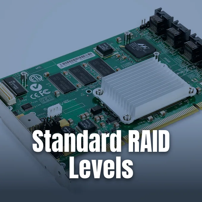
Standard RAID Levels: How Striping, Mirroring, and Parity Work

Standard raid levels combine multiple disk drives into a single logical storage volume to balance input and output speed, fault tolerance, and usable storage capacity [1]. By applying data striping, disk mirroring, or mathematical parity over separate drives, these storage architectures protect computer systems from hardware failures and pool storage resources [2]. In 1987, computer scientists David Patterson, Garth Gibson, and Randy Katz developed this taxonomy at the University of California, Berkeley, demonstrating that coordinated groups of affordable drives could outperform mainframe storage [1]. Modern storage setups balance usable space against workload demands [5].

How Standard RAID Levels Organize Disks

Storage arrays combine member drives through striping, mirroring, and parity [6]. Striping divides contiguous files into separate data units and writes them over independent drives, enabling concurrent read and write commands that raise overall throughput [2]. Mirroring copies data, but parity calculates recovery checksums [7].

In June 1988, Patterson, Gibson, and Katz published their paper, A Case for Redundant Arrays of Inexpensive Disks (RAID), at the SIGMOD Conference in Chicago. The researchers proved that arrays of commodity personal computer disks could outperform single, large, expensive disks (SLEDs) common in mainframe centers [1]. Gus German and Ted Grunau at Geac Computer Corp had earlier explored redundant storage under the name MF-100 [7]. The RAID Advisory Board redefined the acronym in 1992 [1].

Early enterprise vendors deployed redundant arrays before academic papers named them. Digital Equipment Corporation shipped mirrored RA8X disk drives in 1983 as part of its HSC50 subsystem to safeguard mainframe databases. In 1977, Norman Ken Ouchi at IBM filed a patent describing block-level parity, and Clark and other IBM engineers patented distributed parity in 1986 [1]. Storage controllers group these member disks into unified arrays identified by a logical unit number (LUN), building on foundational storage principles of how disk arrays store and protect data in corporate data centers [8]. The Storage Networking Industry Association later codified these formats under the Common RAID Disk Drive Format specification [1].

Striping and Mirroring Tradeoffs

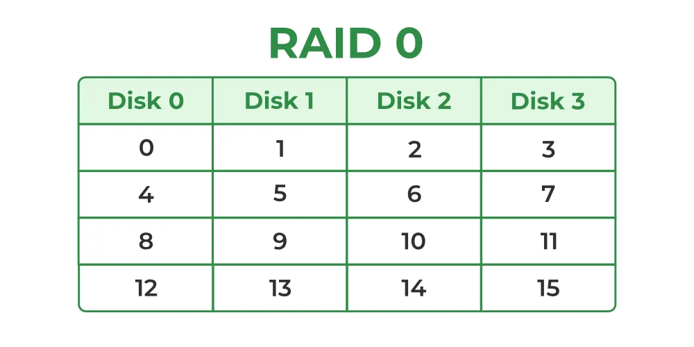
RAID 0 distributes data blocks evenly over two or more drives without parity checksums or duplicate copies [3]. Because the storage controller accesses member disks concurrently, read and write throughput increases with the drive count [11]. It offers zero fault tolerance [5].

The failure probability of a striped array climbs with every drive added to the group. If an individual disk exhibits an annual failure rate of 0.03 (3%), the annual failure rate for a two-drive RAID 0 volume rises to roughly 5.91% [6]. Because losing a single drive destroys all data, administrators avoid it for critical records and deploy it mainly for scratch space, image retouching, and video editing caches where files can be recreated quickly [9].

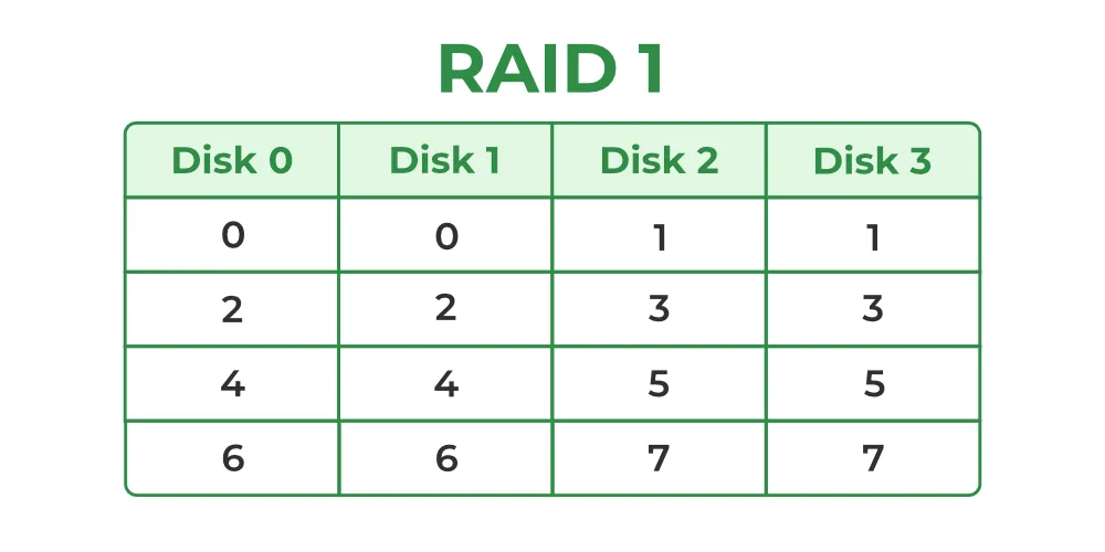
RAID 1 emphasizes complete data redundancy by creating an identical mirror copy of all information on a separate disk [3]. An array needs at least two drives, and the volume continues functioning without data loss as long as one disk remains operational [6]. Because reads can be serviced by either drive, read performance can approach the combined throughput of both disks, but write throughput stays limited to the speed of the slowest drive [3]. For an array of two disks with a 3% single-disk failure rate, the annual failure probability drops to 0.09% [6]. Usable capacity is exactly 50% of the raw space [5].

Dedicated Parity in Early Arrays

To guard against drive failure without surrendering half of raw disk capacity to mirroring, early designs used a single parity disk. Parity calculates a checksum over corresponding data bits using boolean exclusive-OR (XOR) logic. If one drive fails, surviving disks reconstruct the missing information [2].

RAID 2 striped data at the bit level and recorded Hamming-code error-correcting codes on separate parity drives. In 1988, Unisys Corporation secured a patent for a 39-disk RAID 2 array featuring thirty-two data drives and seven error-correction disks [2]. Thinking Machines used an early error-correcting disk array in its DataVault and CM-2 supercomputers, echoing techniques tested on the IBM 353 in the 1960s. Because modern drives incorporate internal error correction, RAID 2 vanished from commercial systems [1].

RAID 3 and RAID 4 refined parity by striping data in bytes and blocks, but both configurations suffered from a severe write bottleneck [2]. RAID 3 synchronizes drive spindles to transfer large sequential files, making it suitable for video workstations but inefficient for database transactions [8]. RAID 4 introduced independent block transfers, allowing multiple read operations to proceed in parallel over separate data disks. NetApp historically used RAID 4 before developing its dual-parity RAID-DP architecture [1]. However, every write command must update the single parity drive, triggering a read-modify-write cycle that requires four disk operations: reading old data and parity, calculating the new parity, and writing both blocks. That single parity disk quickly saturated under transactional workloads [2].

Standard RAID Levels Using Single Parity

RAID 5 resolves the parity bottleneck by distributing checksum blocks evenly over all member disks in the array [2]. In 1986, Clark and colleagues at IBM patented this distributed approach, which became one of the most prominent standard raid levels in server storage [1]. Spreading parity enables all drives to service read requests [2].

A RAID 5 configuration needs at least three drives and provides usable capacity defined by the formula (n – 1) * B, where n is the drive count and B is drive capacity [11]. In a three-drive array, usable capacity reaches 67%, a four-drive array delivers 75%, and a six-drive setup yields 83% of raw storage [5]. The array survives the complete loss of one disk without downtime [7].

Despite distributing parity, RAID 5 still suffers from the read-modify-write penalty during small random writes. Because updating a single block needs reading old data and parity before writing new values, write throughput is lower than mirrored setups. When a drive fails, the array enters a degraded mode where reading lost blocks requires computing parity over all surviving drives [2]. Rebuilding the array puts heavy mechanical strain on remaining disks, leaving the volume vulnerable to total data loss if a second disk fails before reconstruction finishes [5]. Hardware controllers mitigate this write penalty by caching incoming writes in battery-backed memory [6].

Dual Parity and Rebuild Protection

RAID 6 expands distributed parity by generating two independent checksum blocks, commonly designated as P and Q, over every data stripe [2]. The setup needs at least four drives. It provides usable capacity equal to (n – 2) * B, tolerating the simultaneous failure of any two drives [5].

The dual parity scheme uses standard XOR logic for the P parity and Reed-Solomon codes or Galois field mathematics for the Q syndrome [1]. Small random write operations incur a penalty of six disk accesses because both parity blocks must be updated with the new data [2]. Despite this write overhead, RAID 6 has become the standard choice for storage servers holding large spinning drives [5].

Storage consultant Henry Newman examined this shift in Enterprise Storage Forum, showing that hard drive density has outpaced drive bandwidth growth for decades. Drive bandwidth improves by roughly 20% per hardware generation, but drive capacities have grown hundreds of times, causing rebuild times to extend from hours to days. Enterprise SATA drives feature an unrecoverable read error rate of 1 in 10^15 bits, and consumer SATA drives hit unrecoverable errors at 1 in 10^14 bits—equivalent to hitting a read failure every 0.89 petabytes. During a RAID 5 rebuild on multi-terabyte disks, reading entire drives often triggers an unrecoverable read error that destroys the volume [10]. RAID 6 provides the dual-drive tolerance needed to absorb a second drive failure or an unrecoverable read error while the rebuild is underway [5].

Nested Layouts: RAID 10 Versus RAID 50

Nested RAID configurations combine two standard layouts in a layered hierarchy to capture both speed and fault tolerance. In standard naming, the first digit denotes the lower layer and the second digit denotes the top array [4]. RAID 10, or RAID 1+0, stripes data across mirrored stripes using at least four drives [11].

The structural difference between RAID 10 and RAID 0+1 produces major differences in fault tolerance. In an eight-drive RAID 0+1 array, losing a single drive causes an entire striped sub-array to fail, meaning a second drive failure in the other stripe destroys the volume in 4/7 of cases. In an eight-drive RAID 10 array, the volume survives unless the second failing disk happens to be the partner in the same mirrored pair, dropping system failure probability to 1/7 [13].

Rebuilding a degraded RAID 10 array is very fast. Because the storage controller copies data directly from the surviving mirror partner without recalculating parity checksums over other disks, rebuilds finish in a fraction of the time needed for parity volumes [13]. Usable capacity is 50% [8]. For environments needing parity efficiency alongside striping performance, RAID 50 combines block striping over multiple RAID 5 subgroups and needs at least six drives, allowing three RAID 5 arrays of three 120 GB drives to create a 720 GB pool that tolerates one drive failure per subgroup [4].

Selecting Standard RAID Levels for Workloads

Selecting among standard raid levels depends on balancing I/O profiles, usable capacity, and recovery needs [5]. Workloads with frequent random writes suffer under parity recalculations, but read-heavy applications benefit from parallel striping [11]. The right configuration matches specific operational demands [5].

Enterprise database clusters and virtual machine hosts run best on RAID 10 because it eliminates parity calculation penalties and provides high IOPS for concurrent transactions. Although RAID 10 sacrifices half of its raw capacity, the rapid rebuild times and low latency justify the investment for business-critical data, coordinating with infrastructure where service mesh architectures route network traffic between distributed backend services [8]. General file servers and backup staging repositories perform reliably on RAID 5 when limited to small three- or four-drive groups [5].

When disk arrays expand to eight or more large hard drives from manufacturers like Seagate or Western Digital, RAID 6 becomes the necessary baseline to prevent multi-disk failures during lengthy rebuild windows [5]. For small office servers and single-workstation operating systems, RAID 1 provides simple and dependable boot protection over two drives without specialized controller hardware [8]. High-performance rendering stations and temporary caching nodes utilize RAID 0 over two disks to achieve maximum data transfer rates, relying on external network storage for permanent file retention [9]. Storage administrators evaluate these trade-offs to ensure arrays maintain availability without exceeding budget boundaries [5].

Controller Hardware Versus Offline Backups

Storage arrays can be managed through dedicated hardware controllers or operating system (OS) software drivers. Hardware RAID offloads parity calculations to onboard processors, but software RAID uses the host CPU [6]. Both methods present unified volumes to user applications [7].

Motherboard manufacturers brought hardware array support to mainstream computers in 2003 with the Intel ICH5R southbridge on 865 and 875 chipsets, offering two SATA ports with RAID 0 and RAID 1 capability. In 2004, the ICH6R on 915 and 925 chipsets expanded support to four SATA ports, while the ICH7R introduced RAID 5 and Intel Matrix RAID. Motherboards using the AMD SB600, Nvidia nForce 590, and VIA VT8237 southbridges also integrated storage controllers, competing with standalone cards from Promise FastTrak and Adaptec [12]. Dedicated PCIe RAID controller cards with battery-backed cache memory remain standard in high-end servers to absorb parity write delays [6].

Software RAID implementations like Linux mdadm, FreeBSD gmirror, and Windows Server manage arrays efficiently without proprietary hardware controller locks. Advanced file systems such as ZFS combine RAID volume management with cryptographic data checksumming, detecting silent data corruption and automatically repairing corrupted blocks [5]. However, no RAID level replaces a disciplined offsite backup strategy. A RAID array is not a backup. Redundant disk arrays maintain system uptime when a drive fails, but they can’t prevent accidental file deletion, ransomware attacks, file system corruption, or site destruction. When a user deletes a critical database, that deletion instantly propagates across every mirrored and parity disk in the volume [7].

1. ^WEBSITE Wikipedia Contributors. (2026). Standard RAID levels. Wikipedia, The Free Encyclopedia. [Article Link]
2. ^WEBSITE Koren, I. (2010). Basic RAID Organizations. Department of Electrical and Computer Engineering, University of Massachusetts Amherst. [Article Link]
3. ^WEBSITE Wikipedia Contributors. (2026). RAID. Wikipedia, The Free Encyclopedia. [Article Link]
4. ^WEBSITE Wikipedia Contributors. (2026). Nested RAID levels. Wikipedia, The Free Encyclopedia. [Article Link]
5. ^WEBSITE Server Configurator Editorial Team. (2026). RAID Levels Explained: 0, 1, 5, 6, 10 for Servers (2026). Server Configurator. [Article Link]
6. ^WEBSITE Dancuk, M. (2025). RAID Storage: Definition, Types, Levels Explained. Knowledge Base by phoenixNAP. [Article Link]
7. ^{ONLINE NEWS} BasuMallick, C. (2022). What is RAID Storage? Meaning, Types, and Working. Spiceworks Inc. [Article Link]
8. ^{ONLINE NEWS} Posey, B., Sullivan, E., & Peterson, S. (2023). Comparing RAID levels: 0, 1, 5, 6, 10 and 50 explained. TechTarget. [Article Link]
9. ^WEBSITE Laurens. (2020). RAID level 0, 1, 5, 6 and 10 | Advantage, disadvantage, use. Prepressure. [Article Link]
10. ^{ONLINE NEWS} Newman, H. (2009). RAID’s Days May Be Numbered. Enterprise Storage Forum. [Article Link]
11. ^WEBSITE GeeksforGeeks Editorial Team. (2017). RAID (Redundant Arrays of Independent Disks). GeeksforGeeks. [Article Link]
12. ^{ONLINE NEWS} Schmid, P. (2007). The Raid Migration Adventure. Tom’s Hardware. [Article Link]
13. ^WEBSITE Heiss, J. (2009). Why is RAID 1+0 better than RAID 0+1? aput.net. [Article Link]

Cover image: Dmitry Nosachev / Wikimedia Commons, CC BY-SA 4.0